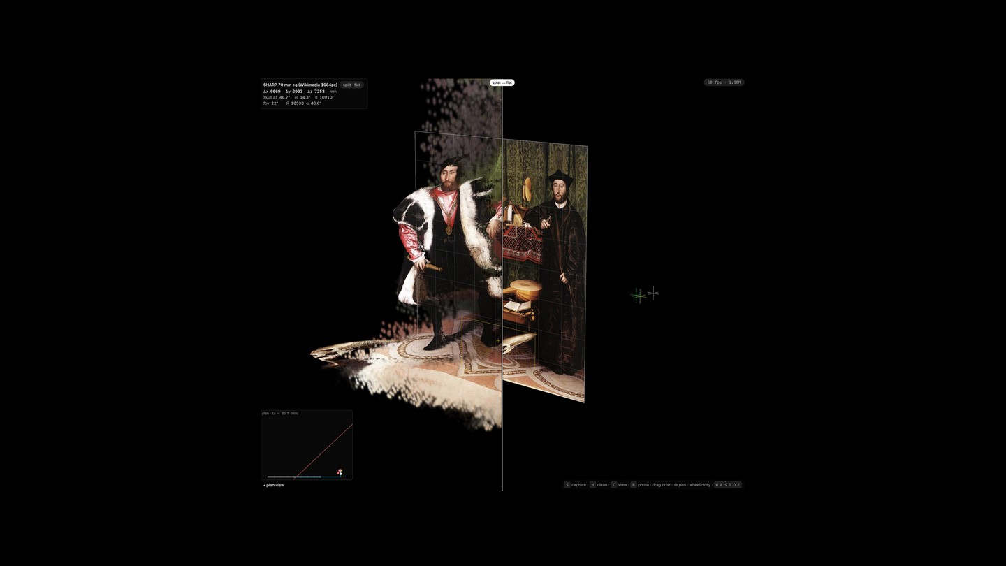
To observe the skull depicted by Holbein, one must stand at a specific vantage point within the Renaissance collection at the National Gallery. This optimal viewing position can be accurately reconstructed from the panel through precise geometrical analysis, achieving millimeter-level accuracy as demonstrated by Idols of the Cave1. However, the objective of this study is to utilize a predictive regression model to perform reverse engineering of the position that most closely approximates the “imaginary position” from which Holbein was situated during the creation of the painting.
01 Coordination
Walter Benjamin, writing in 1936, posited that while a reproduction can disseminate across any geographic location, it inherently lacks the capacity to convey the original's unique presence at a specific place and moment in time. He designated this phenomenon as aura and regarded it as being diminished or lost through mechanical reproduction processes2.
Holbein's The Ambassadors (1533) presents a compelling case study for analyzing the concept of aura. The depiction of the skull within the lower panel appears as a smudged image that becomes perceptible only from an oblique viewing angle to the right of the composition. A straightforward photograph of the painting fails to reliably reproduce the skull, because the perception of the skull does not solely reside in the mechanical transition from pigments to pixels. Instead, it emerges within the experiential context of the viewer's perception at the precise “moment of originality”3. The Ambassadors exemplifies this ephemeral quality of the “here and now,” which necessitates specific spatial and perceptual coordinates during the act of viewing.
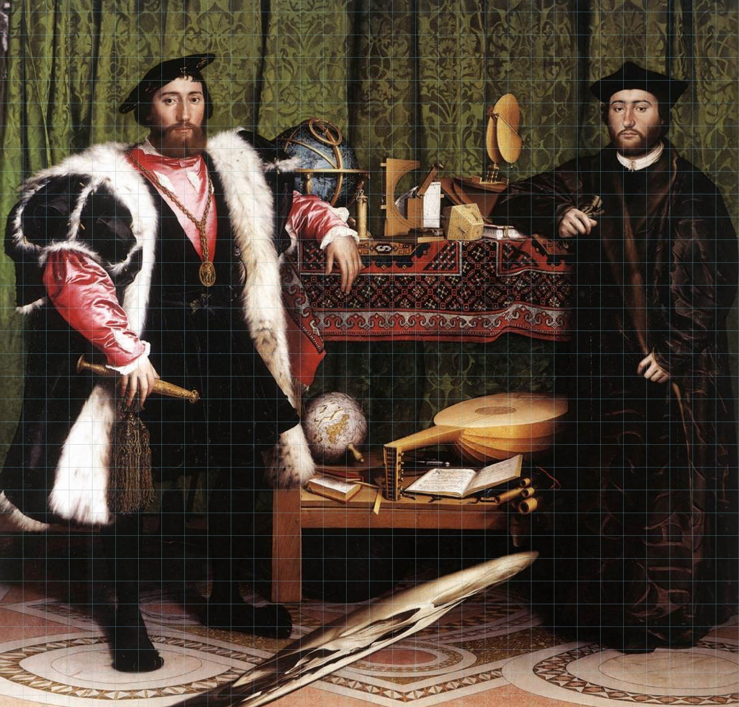
This analysis draws methodological inspiration from Boxer's approach, applying solely geometric analysis through an “inverse trapezoid” transformation1. This technique reconstructs the formation and assesses the extent to which an observer's gaze can drift before the skull ceases to be perceptually resolvable. Additionally, the SHARP neural network — designed to convert a single photographic image into a metric 3D scene4 — is employed to investigate the same perceptual phenomena from a computational perspective.
02 Simulation
For Baudrillard, simulation is distinguished from pretense5. He employs an illustrative example that I find particularly enlightening: an individual feigning illness remains healthy; the pretense exists externally, and an examination can detect the falsehood. Conversely, a person engaging in simulation of illness produces genuine symptoms, rendering the examination unable to differentiate between reality and simulation. This conceptual experiment can be extended to our context to question what we actually perceive when we “see” — are we merely engaging in pretense, since we are essentially receiving light stimuli through the retina, or is the act of seeing itself a form of mental simulation mediated by neural processes within the brain?
Baudrillard larger claim extends this to representation itself. Once models are cheap, detailed and everywhere, the copy stops depending on an original and begins standing in for it. A model that has displaced its referent is referred to a simulacrum; the condition it produces is called hyperreal, meaning not false but no longer answerable to anything outside itself.
An anamorphosis is a rare object that keeps its outside: the correct viewing position is recoverable from the panel independently of any model, with a published uncertainty attached. The model can therefore be caught — and the interesting work is catching it precisely enough that the disagreement means something.
Douglas Davis argues that the aura does not die in the copy but relocates into the individual act of looking, wherever the image is met3. Between the three positions sits one testable question. If the moment of seeing has a location, can an instrument find it?
Another noteworthy observation is that the resolution of the image used in this experiment is 1084 x 1069 pixels, which constitutes a relatively limited pixel count for optimal performance in a regression model. Additionally, this raises concerns regarding the effective resolution reduction from the original physical artwork, which exists at an atomic scale. The artwork is scaled down to merely 1,158,796 pixels, equivalent to approximately 1.16 megapixels. This diminution of detail contributes to an additional layer of information loss, thereby impacting the overall dissimilarity measure. The subsequent step would involve evaluating the employment of the high-resolution version scanned by Google Art Project.

03 Error and Bias
In Troika's Ghost Specimen, the artists began with a pressed herbarium sheet of a flower that had been extinct for a century. Pressing keeps one flat aspect of the organism and destroys the other. Asked to reconstruct the whole plant, a generative image model produced the missing face from the statistical regularities of every other specimen it had seen. The result, which joins the original pressed specimen to the generated face, was then exhibited on a wall, where the model's “imperfection” was no longer visible6.
An earlier precedent for this experiment is the visualisation of fluid-dynamics data by electromechanical plotters at Los Alamos in the 1950s and 1960s, as recorded in the laboratory's reports7. Those drawings let scientists study shockwaves and high-velocity collisions, conditions under which solids deform, liquefy or vaporise, without running the physical experiment. A series of drawings was produced from cumulative calculation, so that phenomena and spatial configurations that could not be realised physically could still be pictured and examined.
Both projects work at the boundary between the real and the artificial. When a machine meets incomplete or ambiguous information it is built to produce a plausible reconstruction, which is to say that it hallucinates, and the reconstruction carries the biases of its training data and of its architecture. It is fair to ask, for example, whether the weighting inside a deep network favours some kinds of image over others. Authorship and agency become harder to locate. In this experiment three agents, Holbein, the regression model and myself, negotiate a shared agency across three different perceptions of what is real.
04 Premise
Boxer's construction uses five points marked on the anamorphic skull, measured in millimetres from the panel's lower-left corner, plus two conditions on the restored image: the jaw line becomes horizontal, and the restored skull fits a square. Eye height is fixed at the panel's midline, which the painting's own perspective supports. With the panel at 2095 × 2070 mm after the restoration record8, the viewing point lands at Δx = 776.9 mm right of the panel's right edge, Δy = 1035 mm above its bottom edge, Δz = 257.9 mm off the wall, with a stated uncertainty of 20 × 4 mm. The National Gallery's own figure, found by adjusting the image in a graphics program until the skull looked right, is (790, 1040, 120)9.
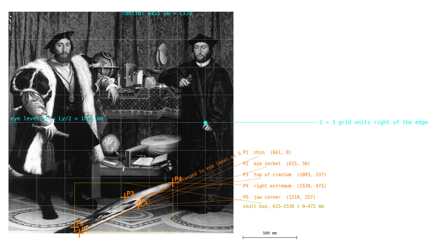
A Python port of Boxer's two MATLAB scripts returns every published number to within 0.2 mm. The port also shows how little the construction depends on. The horizontal-jaw condition requires only that the jaw line pass through S, which fixes D = 1824.45 mm in a single line; the square condition is a ratio, which fixes d = 257.88 mm.
The same transparency shows where the construction rests. The whole result depends on one judgement, that a painted jawbone is a straight line, and Boxer says so himself. The method is exact, but it is exact about a premise that cannot be checked against the panel.
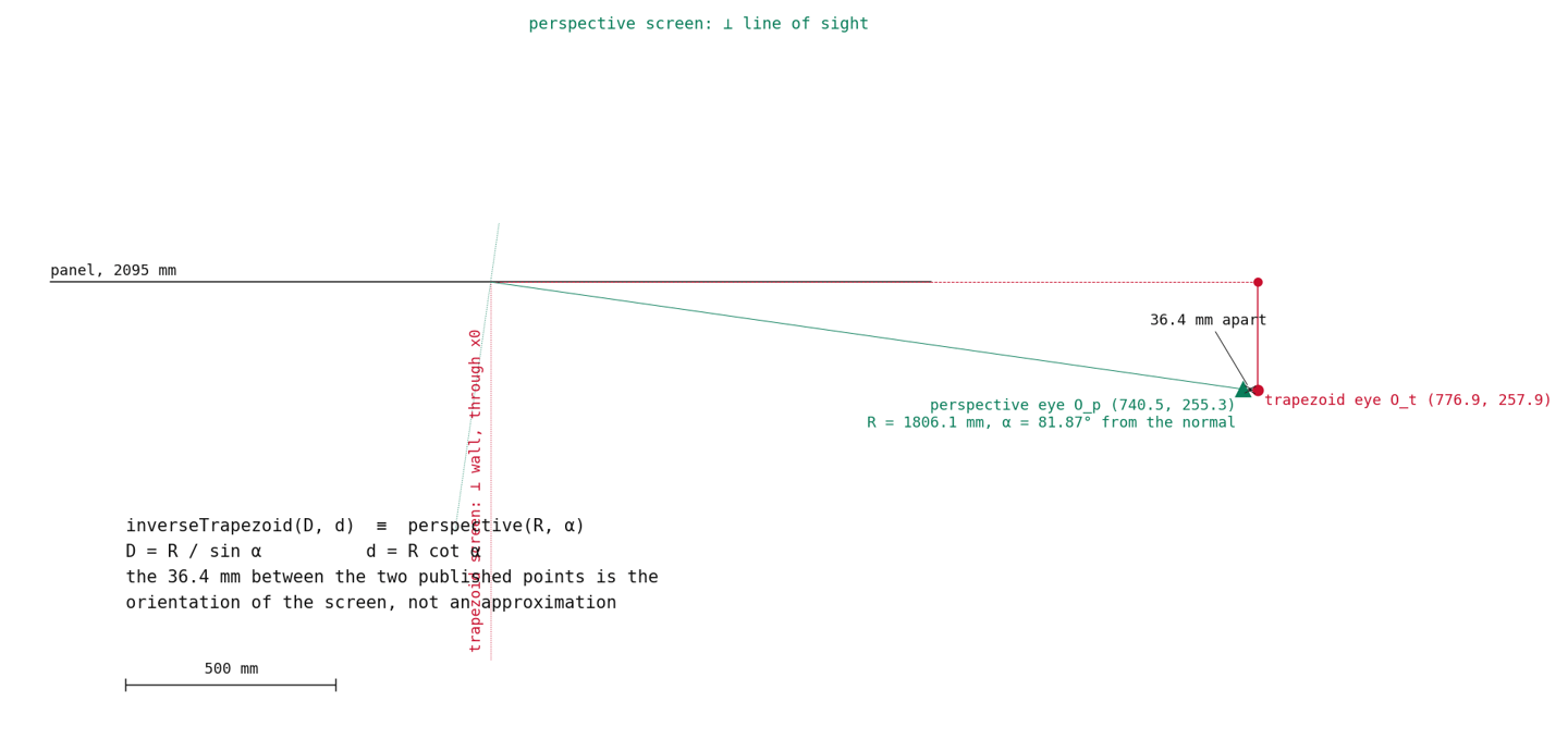
The port also corrected a misunderstanding in this study's own brief rather than anything in Boxer's work. His two transforms are not approximations of one another; they are the same function. Perspective projection at distance R and angle α equals the inverse trapezoid with D = R / sin α and d = R cot α, identically. The 36 mm between his two published points is the orientation of the screen the image is projected onto, not an error. At the millimetre scale, "the" viewing point is already a convention before any model is involved.
05 How wide is “it looks like a skull”?
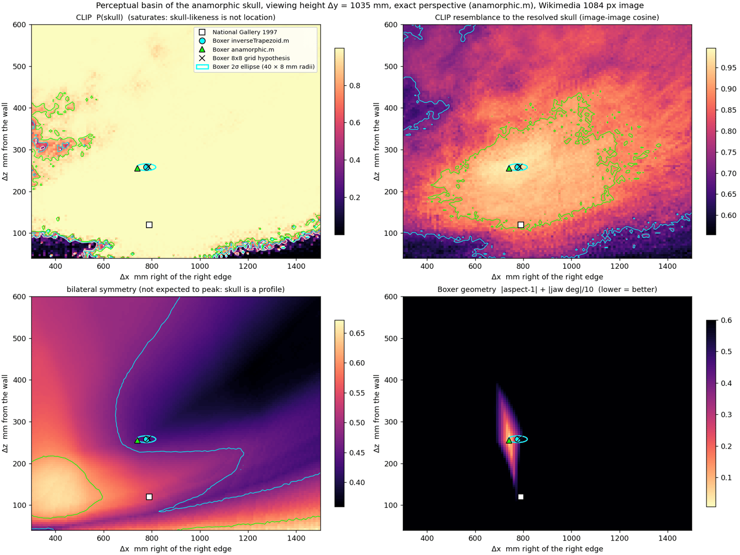
Before asking a model for the position, the flat painting was projected from 13 700 eye positions on a 10 × 5 mm grid at eye height, and each skull crop scored with CLIP, a network that rates how well an image matches a phrase10. "A human skull" scores above 0.99 almost everywhere. A skull stretched to twice its length is still a skull to the network, and the region within 5 % of the best score covers 604 times the area of Boxer's ellipse. A stricter score, image-to-image similarity against the resolved skull itself, still leaves a basin 24 times that ellipse.
Perception places the viewer somewhere in a large region of acceptable smears; geometry places them within a few millimetres.
These are different kinds of answer, and the study keeps them apart rather than splitting the difference. This is also the quantitative form of Boxer's objection to the National Gallery's method: adjusting the image until it looks right cannot be more precise than the tolerance of looking, and that tolerance turns out to be very wide.
06 Invented Depth
SHARP was given the same photograph. When an image carries no camera data the model assumes a 30 mm lens and reports depth in metres derived from that assumption. There was no lens in 1533, so every metre the model returns rests on a default.
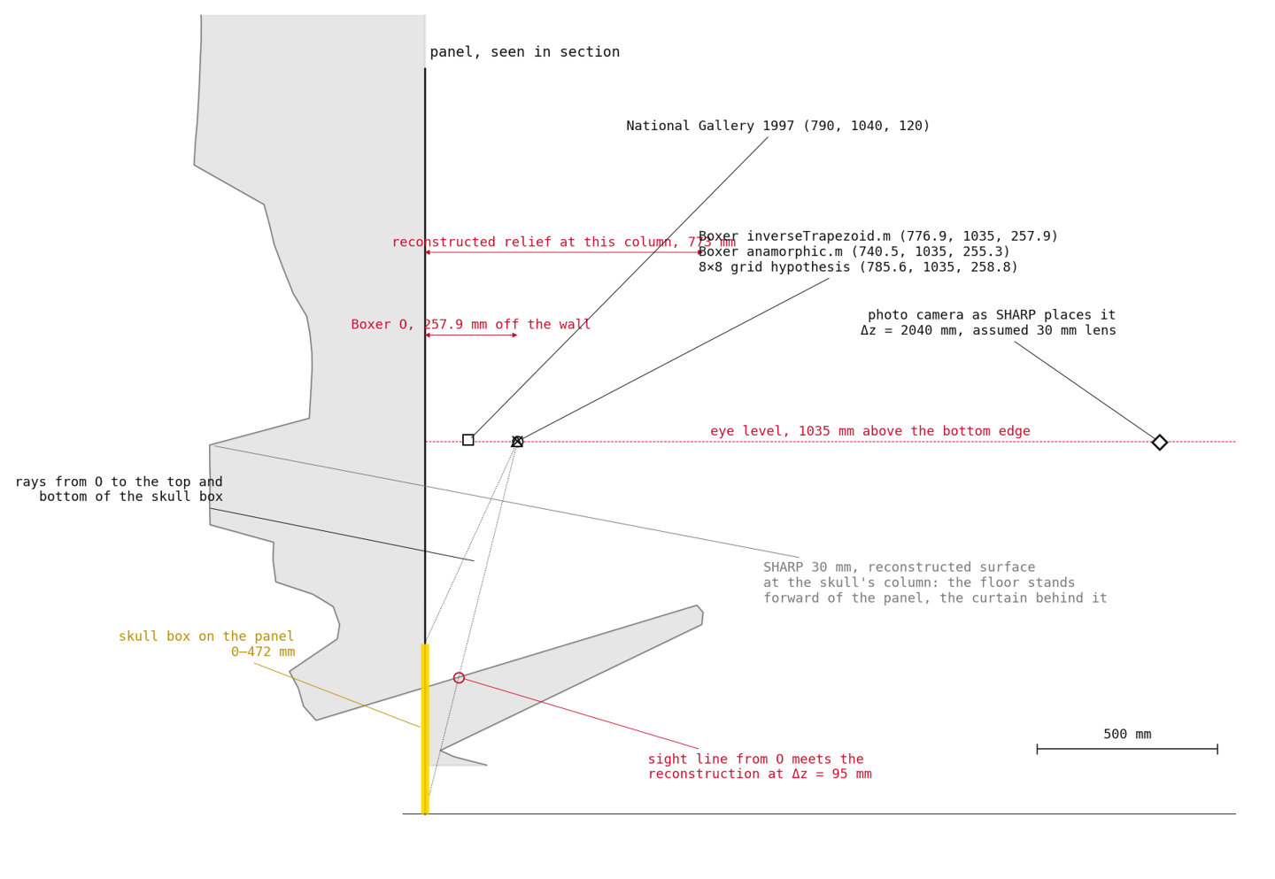
The model did not reconstruct a panel; it reconstructed the room the painting depicts. The floor advances, the curtain recedes, and 623 mm of relief appear across a surface 2095 mm wide that is physically flat. A plane fitted to the image border tilts by twenty degrees, because the bottom border is the depicted floor.
Comparing metres to millimetres therefore requires deciding where the panel is, and that decision is a stated assumption rather than a hidden one. The primary bridge places a plane parallel to the photograph at the reconstructed depth of the skull and sets its width to 2095 mm; a global-median plane and the tilted border fit are carried as bounds. One SHARP metre then equals 1095 mm, the photograph's own camera stands 2.04 m from the wall, and the skull's known 915 mm width returns as 1036 mm per metre, a 6 % check. The bridge is unit-tested against a synthetic plane and written into every render. It is the weakest link in the study, and for that reason it is kept in view.
07 Resection
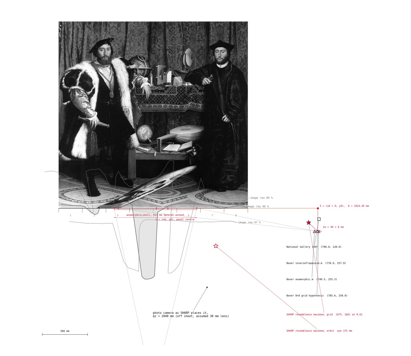
In photogrammetry, resection means recovering a camera's position from what it saw. The model's scene was photographed from 1421 positions on the same grid as the perceptual sweep, looking horizontally at the panel's centre as in Boxer's script, and from a 532-position orbit around the skull.
The scoring crop cannot be placed where the flat panel puts the skull, because that box comes back almost empty: the model has not placed the skull on the wall. The crop instead follows the projected 3D bounding box of the Gaussians belonging to the skull in the photograph11. At Boxer's O that box is 87 % empty.
Resemblance across the whole grid stays between 0.30 and 0.61, below what the flat panel scores even at the National Gallery's point, and its maximum sits 141 mm from Boxer's O, at (675, 1035, 160). Measured against the disagreement between the two human estimates (13 mm along the wall, 138 mm out from it), that is eight units off along the wall and less than one unit out from it. That number is not a station point in Boxer's sense; it is the best available view of a streak lying on a receding floor.
08 Phantom Lens
Since every metre descends from a default, the default was swept from 5 to 200 mm. Depth is exactly linear in the assumed focal length and the lateral scale does not move: the model's metric guess is a depth guess only, and relief follows it, from 104 mm at 5 mm to 4.1 m at 200 mm. No lens brings the model's best position inside the ellipse.
A short lens flattens the scene, and at 5 mm, from Boxer's exact-perspective point with a narrow field of view, the skull begins to read. This is suggestive rather than conclusive: it is a single capture, the scoring crop misses it because the crop sits at the wrong depth, and a 5 mm equivalent lens is not a plausible camera. What it does show is where the obstacle lies. The lens prior is what stands between the model and the panel.

09 Idolmorphosis
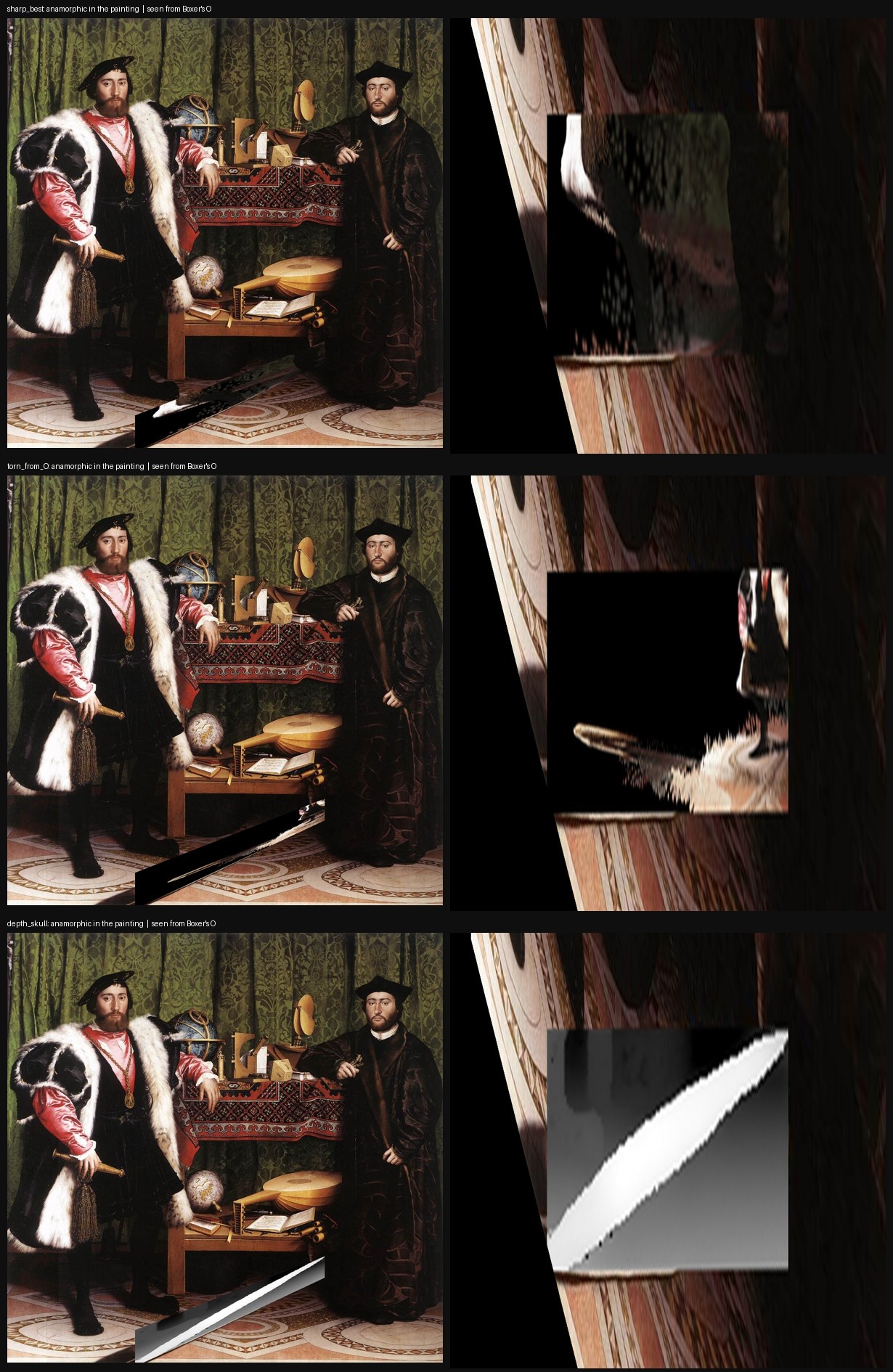
Boxer ends by running his procedure backwards: a square image placed in the 142 mm box of the restored painting and forward-transformed with the same D and d lands exactly where Holbein's skull lies. The same was done here with the model's output: its best crop, its torn render from O, and its depth map of the skull region. Each becomes a 914 × 532 mm streak, saved at four pixels per millimetre for a 36-inch print, that resolves only from the exact-perspective point.
The depth map reads best from O: the model's estimate of where the skull is, stretched across the floor where Holbein stretched the skull. Whether that is an artefact or a diagram is a question the print leaves to the visitor who walks up to it.
10 The Outside
The geometer's answer is the viewpoint saved in this instrument as the resolved skull: (740.5, 1035, 255.3) mm, R = 1806 mm, 81.9° from the wall normal, where the flat panel scores 0.997 and Boxer's construction reproduces to a hundredth of a millimetre. The model's answer is not a small error; it is an answer to a different question. Given a photograph with no lens it fills in a room, and once there is a room, the floor carries the smear away from the wall on which the construction depends.
This is the useful result, and it runs against the theory it was meant to illustrate. Baudrillard's model does not pretend to see a skull; it produces the symptoms of a scene, and those symptoms are coherent enough to be measured. They were measured, and at a specific coordinate they were found wanting. The hyperreal is supposed to have absorbed its outside. Here the outside held, not because the model is weak but because the object was chosen so that a physical fact remained recoverable.
On this evidence, the precession of simulacra is less a property of models than of situations in which nothing remains to check them, and such situations are arranged rather than given.
Benjamin's aura did not stay in the panel, and it did not pass to the model. It sits in the bridge, the list of assumptions that allow millimetres to be compared with metres. Davis is right that the moment of seeing survives reproduction; here it survives as a coordinate that someone has to argue for, and that argument is the work.
11 Objections
Four objections, in descending order of how much weight they carry against the result.
- The judge is a network. Resemblance is scored by CLIP, which carries its own biases and was trained on the same kind of internet imagery as the model under test. A network is being asked whether another network's output looks like a skull. This was accepted because a human judge would be the thing under test, but it means that every score in §05 and §07 compares two priors rather than reporting a perceptual fact.
- The bridge is chosen, not derived. Three defensible bridges disagree by up to 25 % in scale. All three were carried and the conclusion holds under all three, but a reader who rejects the primary bridge is entitled to reject the specific millimetre figures that depend on it.
- Boxer's premise cannot be tested against the panel. The construction assumes that the painted jawbone is a straight line, and nothing in the object can confirm it. The ground truth is a precise consequence of a reading that cannot itself be checked.
- The comparison is unfair by design. SHARP was not built to solve anamorphosis; it was built to produce plausible geometry from one photograph, and by that standard it succeeds. The test is not one of competence. It asks what a model does with a question it cannot know it is being asked, and whether the answer arrives marked as a guess. It arrives, instead, in metres.
None of the four touches the central observation, which depends on no metric at all: at the one position where the geometry resolves the skull, the model has nothing on the wall.
12 The Instrument
The interface is not an illustration of this study. It is the apparatus the measurements were taken with, and every figure above can be reproduced from it. It holds one painting, several reconstructions of it, and three coordinate frames kept deliberately separate. Lab is the instrument, Log is its record, Report is its running summary.
The three frames
Every number in the app belongs to exactly one of these frames; the bridge exists so that they are not confused.
| Frame | What it holds |
|---|---|
| Panel (mm) | The physical frame, and the one the argument is conducted in. Δx = millimetres right of the panel's right edge, Δy = above its bottom edge, Δz = out from the wall. The panel is 2095 × 2070 mm. |
| SHARP (m) | The model's own frame, in metres, x right, y down, z forward from the photograph's camera. These metres are not measurements; they are consequences of an assumed lens. |
| Bridge | The stated conversion between the two, as mm per SHARP unit. It is an assumption, it is recorded in every capture, and it is the number most likely to invalidate a comparison if it is wrong. |
The controls
| Control | What it does |
|---|---|
| Scene | One reconstruction: the photograph passed through SHARP at one assumed lens. Reference scenes are the thirteen lenses of the sweep; Tests are reconstructions made from views rendered inside the app. The badge shows the lens. |
| View | How the loaded scene is drawn, camera held fixed so the five are comparable. Splat: the 1.18 million Gaussians. Mesh: the depth map as a textured surface. Wire: the same depth as lines, which makes invented relief legible. Flat: the painting on a flat panel from the same camera, which is Boxer's model and the control condition. Split: splats against one of the others. |
| Viewpoints | Named eye positions on keys 0–5: the camera the model assigns to the photograph, the four published estimates, the reconstruction's own scoring maximum, and anything saved in session. Selecting one sets Δx, Δy, Δz and field of view together. |
| Trajectories | Camera paths between positions, so a claim about a region can be shown rather than sampled: the approach to O, sweeps along Δx and Δz, a descent, the orbit, a grazing pass. Record writes every frame plus an mp4 to the Log. |
| Overlays | Construction geometry drawn into the 3D scene rather than painted over it, so it occludes correctly and shows where the reconstruction sits relative to the panel: the 8 × 8 grid, skull box, station points, Boxer's S–O construction, sight lines, depth wireframe. |
| Capture | Writes the frame as a JPEG beside a JSON sidecar holding the pose in both frames, field of view, view mode, active overlays and bridge parameters. The filename repeats scene, view, pose, field and tag, so a capture stays identifiable detached from its sidecar. This is what lets a screenshot stand as evidence. |
| Reconstruct | Renders the painting from the current camera and runs SHARP on that render, passing the render's true focal length. The result enters as a Test scene, bridged from the render camera rather than assumed, the one way to feed the model an image whose lens is known. |
The numbers
| Reading | What it is |
|---|---|
| Δx Δy Δz | Current eye in panel millimetres. Boxer's O is (776.9, 1035, 257.9); the resolved-skull viewpoint is (740.5, 1035, 255.3). |
| az · el · d | Direction from eye to skull: azimuth from the wall normal, elevation, distance in mm. Grazing views, which the model tends to favour, show high azimuth and negative elevation. |
| fov | Field of view in degrees. It sets how much of the smear is in frame, and the 5 mm result in §08 depends on it. |
| R · α | Boxer's own two parameters, recomputed live: R the distance from eye to panel centre, α the angle from the wall normal. At his solution, R = 1806 mm, α = 81.9°. |
| f_px | The assumed focal length in pixels for this scene, the origin of every metre that follows. |
| Relief | Depth p95 minus p05 in panel millimetres: how much depth the model has added across a flat board. 623 mm at the 30 mm default. |
| mm per unit | The bridge, stated. 1095 at the default lens. |
| Grid peak · Offset | Best-scoring position on the resection grid, and its distance from Boxer's O. 141 mm at the default lens, the study's main disagreement. |
Notes
- Source image:
Holbein-ambassadors.jpg, 1084 × 1069 px, the Wikimedia file Boxer worked from. Panel dimensions after the 1996 restoration8. - All measurements, including those that failed, are recorded in
anamorph/findings.md. Figures are drawn bymethod_figures.py; their drawing conventions follow the retroactive-photogrammetry plates in12. The reproduction of Boxer's scripts is inanamorph/boxer_repro/. - Model weights and inference code: github.com/apple/ml-sharp. Every run in this study used the released checkpoint with no fine-tuning.
- Method, Log, Report and the Lab run from published files with no model installed; reconstructing a new view needs the SHARP checkpoint on a local machine.
Further reading: Baltrušaitis, J. (1977) Anamorphic art, trans. W.J. Strachan; Kircher, A. (1646) Ars magna lucis et umbrae, the trapezoid construction Boxer inverts.
References
-
Boxer, A. (2012) ‘Anamorphic Ambassadors’, Idols of the Cave, May. Available at: idolsofthecave.com (Accessed: 9 September 2026). ↩ ↩2
-
Benjamin, W. (1968) ‘The work of art in the age of mechanical reproduction’, in Arendt, H. (ed.) Illuminations. Translated by H. Zohn. New York: Schocken Books, pp. 217–251. Originally published 1936. ↩
-
Davis, D. (1995) ‘The work of art in the age of digital reproduction (an evolving thesis: 1991–1995)’, Leonardo, 28(5), pp. 381–386. ↩ ↩2
-
Mescheder, L., Dong, W., Li, S., Bai, X., Santos, M., Hu, P., Lecouat, B., Zhen, M., Delaunoy, A., Fang, T., Tsin, Y., Richter, S.R. and Koltun, V. (2025) ‘Sharp monocular view synthesis in less than a second’, arXiv:2512.10685. Available at: arxiv.org/abs/2512.10685. ↩
-
Baudrillard, J. (1994) Simulacra and simulation. Translated by S.F. Glaser. Ann Arbor: University of Michigan Press. Originally published 1981. ↩
-
Troika (n.d.) Ghost Specimen. Available at: troika.uk.com (Accessed: 9 September 2026). ↩
-
Harlow, F.H. and Fromm, J.E. (1965) ‘Computer experiments in fluid dynamics’, Scientific American, 212(3), pp. 104–110. ↩
-
Wyld, M. (1998) ‘The restoration history of Holbein’s Ambassadors’, National Gallery Technical Bulletin, 19, pp. 4–25. ↩ ↩2
-
Foister, S., Roy, A. and Wyld, M. (1997) Making and meaning: Holbein’s Ambassadors. London: National Gallery Publications, p. 53. ↩
-
Radford, A., Kim, J.W., Hallacy, C., Ramesh, A., Goh, G., Agarwal, S., Sastry, G., Askell, A., Mishkin, P., Clark, J., Krueger, G. and Sutskever, I. (2021) ‘Learning transferable visual models from natural language supervision’, Proceedings of the 38th International Conference on Machine Learning, PMLR 139, pp. 8748–8763. ↩
-
Kerbl, B., Kopanas, G., Leimkühler, T. and Drettakis, G. (2023) ‘3D Gaussian splatting for real-time radiance field rendering’, ACM Transactions on Graphics, 42(4), pp. 1–14. ↩
-
Pearce, T. (2024) ‘Measuring Adolf Loos’ parallax: retroactive digital photogrammetry and the persistent off-screen’, ARENA Journal of Architectural Research, 9(1): 5. ↩